|
|
2 years ago | |
|---|---|---|
| .idea | 2 years ago | |
| 0.5Mb | 2 years ago | |
| 8000Mb | 2 years ago | |
| RED | 2 years ago | |
| Test | 2 years ago | |
| images | 2 years ago | |
| img | 2 years ago | |
| logo | 2 years ago | |
| question5 | 2 years ago | |
| sim | 2 years ago | |
| traceanalyzer | 2 years ago | |
| 1- Group Guide.pdf | 2 years ago | |
| 2- Group work Contract.pdf | 2 years ago | |
| 3- Installation-updated.pdf | 2 years ago | |
| 4- ns2.pdf | 2 years ago | |
| 5- TCP Flavours.pdf | 2 years ago | |
| 123.sh | 2 years ago | |
| README.md | 2 years ago | |
| analyser.py | 2 years ago | |
| analyser2.py | 2 years ago | |
| cubic.nam | 2 years ago | |
| cubicCode.tcl | 2 years ago | |
| cubicTrace.tr | 2 years ago | |
| data.csv | 2 years ago | |
| plot_RED.ipynb | 2 years ago | |
| reno.nam | 2 years ago | |
| renoCode.tcl | 2 years ago | |
| renoTrace.tr | 2 years ago | |
| vegas.nam | 2 years ago | |
| vegasCode.tcl | 2 years ago | |
| vegasTrace.tr | 2 years ago | |
| yeah.nam | 2 years ago | |
| yeahCode.tcl | 2 years ago | |
| yeahTrace.tr | 2 years ago | |
README.md
Abstract
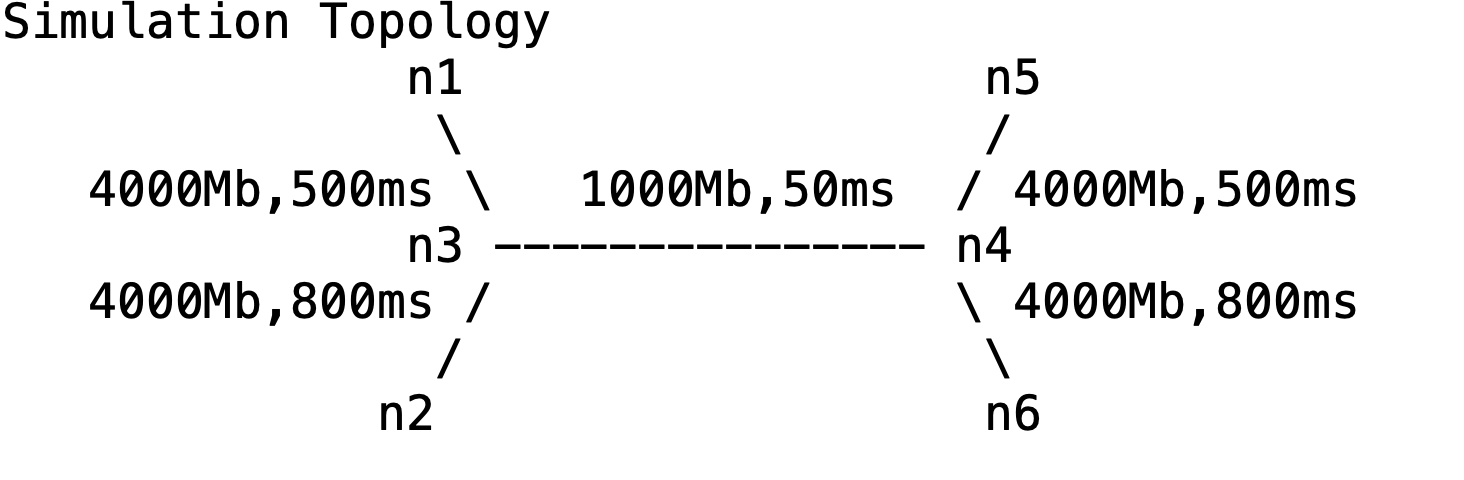
This experiment uses ns2 to construct a simulation scenario comprising
one node and five different line bandwidths and latency. Specifically,
N3 and N4 nodes serve as a router to connect the networks. The queue
size from N3 to N4 is 10. From the network topology, the bandwidth
of link N3 \sim N4 is the network’s bottleneck. In fact, the main
factors that influence the performance the queue size and network
latency. In our experiments, we analyze the factors of 4 TCP
congestion control algorithms that could impact the packet loss,
Goodput rate and end-to-end delay. Moreover, we adjust the parameters
of the experiments to demonstrate the reasonability of our proposed
assumptions. Meanwhile, we compared the performance of RED and
DropTail. Then we further analyze the reasons for such different
performances of RED and DropTail. Furthermore, we conduct experiments
to determine the best fit scenario of RED and DropTail.
Project Introduction
Part A: Experimental Environment Setup
Preparing the Ubuntu OS as a virtual machine
-
Download and install VMWare workstation
-
Download the Ubuntu ISO image.
-
Create a new virtual machine in VMWare and set memory size (RAM) to 2048 MB.

Create a new virtual machine 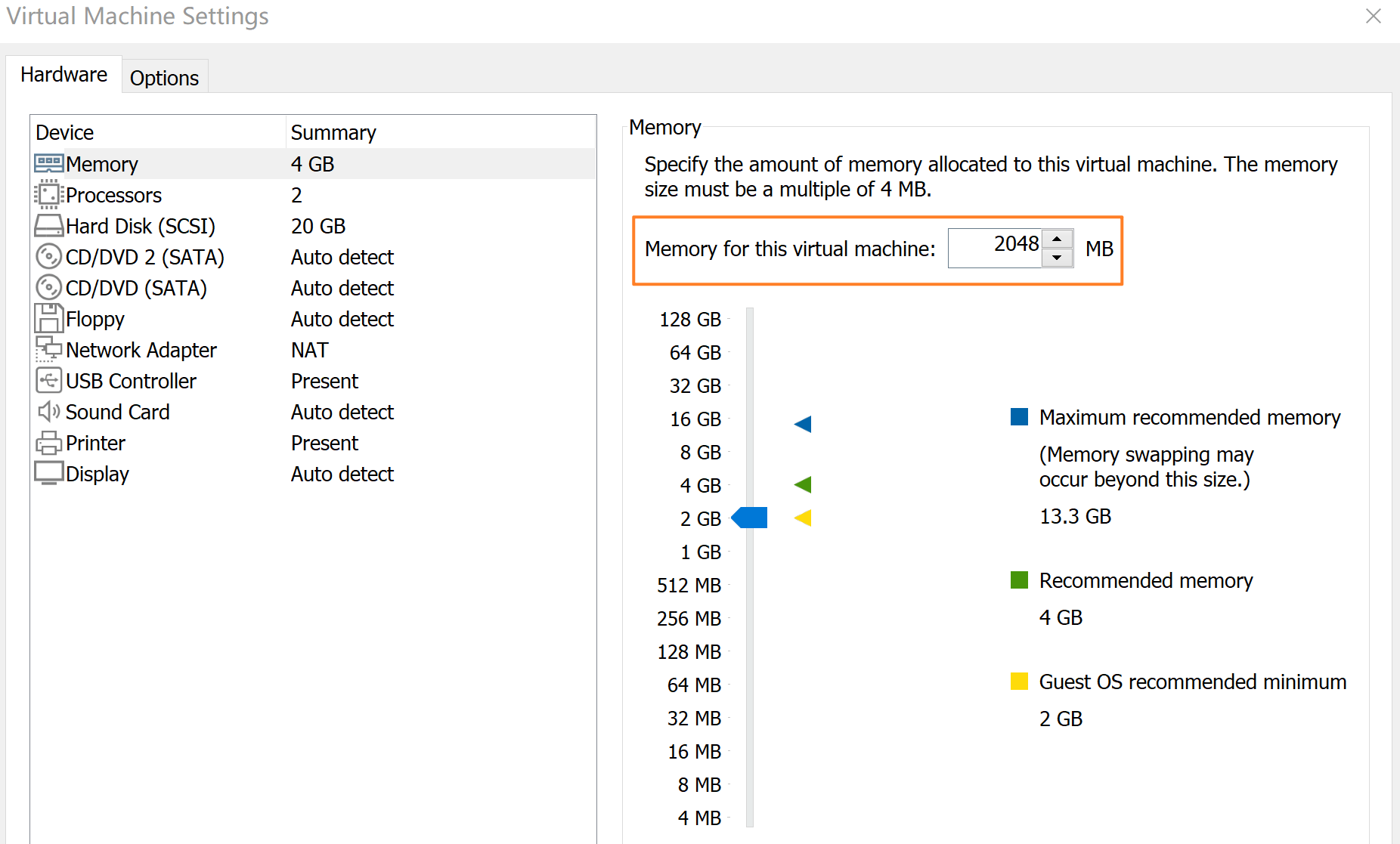
Memory size Analyze -
Create virtual hard disk and select VDI type of hard disk file and dynamically allocated hard disk file size.
-
Set 20 GB of file size. When the virtual machine is ready - set 2 CPUs, and the video memory to 128MB in the Display tab.
-
Install Ubuntu system
NS2 Installation


-
Install ns2, NAM (Network Animator), and Tcl (Tool Command Language) and verify the installation of ns2
-
Clone the project Git repository and Run the test file
Part B: Network Simulator Setup
Trace File, Trace Data Analyzer Script and Plotting
The trace file, which may contain hundreds of lines, records the simulation’s outcome in the event’s format. Consequently, we use scripting languages such as awk or Python to extract meaning (analyze) from the trace file.
     cat out.tr | // Read out.tr file and pipe the output to the next command
     grep " 2 3 cbr " | // Look for 2 (from) 3 (to) cbr (type) line
     grep ^r | // Select lines start with letter 'r' (receive)
     column 1 10 | // Select column 1 - 10
     awk '{dif = $2 - old2; // check whether there is a different in time
        if(dif==0) dif = 1;
        if(dif > 0) { // calculate jitters
            printf("%d\t%f\n", $2, ($1 - old1) / dif); old1 = $1; old2 = $2}
        }'
     > jitter.txt // REDirect output to 'jitter.txt'
Python library to Analyze .tr files


TCP Congestion Control Algorithm Simulation
Why does the plot look very unstable at the beginning of the simulation?
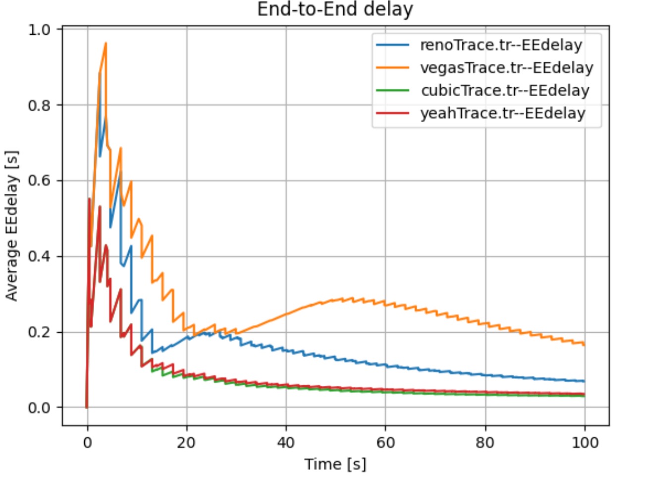
End-to-End Delay
It is important to note that the End-to-End Delay measured at the N4
node changes steeply with time (see Figure
1 and Figure
2). We propose two reasons for
that steep change. Firstly, there is some time difference between
each send due to delayed ACK response. Secondly, two sources may
affect the end-to-end delay. One source is packets from N1 with a delay
of 500ms + 50ms. Another source is packets from N2 with a delay of
800ms + 50ms. To demonstrate our supposition’s validity, we conducted
the following comparison experiments.

For one thing, there is some time difference between each send. This is because senders should wait until ACK is received or timeout and then send a new packet. This includes an extra waiting time. All of these reasons may affect the end-to-end delay.
For flow 1 (from N_1 to N_5),
T_{odd} =\underbrace{T(N_1 \sim N_3) + T(N_3 \sim N_4)}_{Sending}T_{even} = \underbrace{T(N_4 \sim N_5)}_{Sending} + \underbrace{T(N_5 \sim N_4) + T(N_4 \sim N_3) + T(N_3 \sim N_1)}_{Waiting ACK \downarrow} + \underbrace{T(N_1 \sim N_3) + T(N_3 \sim N_4)}_{Next~Sending}For flow 2 (from N_2 to N_6),
T_{odd} = \underbrace{T(N_2 \sim N_3) + T(N_3 \sim N_4)}_{Sending}T_{even} = \underbrace{T(N_4 \sim N_6)}_{Sending} + \underbrace{T(N_6 \sim N_4) + T(N_4 \sim N_3) + T(N_3 \sim N_2)}_{Waiting ACK \downarrow} + \underbrace{T(N_2 \sim N_3) + T(N_3 \sim N_4)}_{Next~Sending}Thus, the difference for these two measured time is
T(N_4 \sim N_5) + \underbrace{T(N_5 \sim N_4) + T(N_4 \sim N_3) + T(N_3 \sim N_1)}_{Waiting ACK \downarrow}
for flow 1 and
T(N_4 \sim N_6) + \underbrace{T(N_6 \sim N_4) + T(N_4 \sim N_3) + T(N_3 \sim N_2)}_{Waiting ACK \downarrow}
for flow 2.
| Time (s) | Event | Packet No. | E-E Delay (\frac{cum\_interval}{samp}) |
Accumulated Interval | Sample |
|---|---|---|---|---|---|
| 0 | TCP From N1 | 1 | 0 | 0 | 0 |
| 0.50 | Packet 1 @ N3 | 1 | / | 0 | 0 |
| 0.55 | Packet 1 @ N4 | 1 | \frac{0.55}{1} = 0.55 \uparrow |
0.55 | 1 |
| 1.05 | Packet 1 @ N5 | 1 | / | 0.55 | 1 |
| 1.55 | ACK @ N4 | 1 | / | 0.55 | 1 |
| 1.60 | ACK @ N3 | 1 | / | 0.55 | 1 |
| 2.10 | ACK @ N1 | 1 | / | 0.55 | 1 |
| 2.10 | TCP From N1 | 2 | / | 0.55 | 1 |
| 2.60 | Packet 2 @ N3 | 2 | / | 0.55 | 1 |
| 2.65 | Packet 2 @ N4 | 2 | \frac{2.65}{2} = 1.325 \uparrow |
2.65 | 2 |
Waiting Time (Waiting for ACK)
For another, we use the following codes to show how the E-E delay changes with time if we include only one source. The first below block closes the N2 source, and the second below block closes the N1 source.
//$ns at 0.0 "$myftp2 start"
$ns at 0.0 "$myftp1 start

$ns at 0.0 "$myftp2 start"
//$ns at 0.0 "$myftp1 start
When we only include a single source, the trends change regularly, which is different to our previous random and steep changes (see Figure 4).

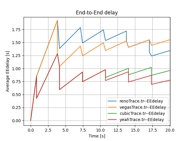
Now we take the Reon TCP congestion control algorithms as an example, which also applies to other congestion control algorithms.
| Time (s) | Event | Packet No. | E-E Delay (\frac{cum\_interval}{samp}) |
Accumulated Interval | Sample |
|---|---|---|---|---|---|
| 0 | TCP from N1 | Packet 1 | / | 0 | 0 |
| 0 | TCP from N2 | Packet 2 | / | 0 | 0 |
| 0.5 | Packet 1 @ N3 | Packet 1 | / | 0 | 0 |
| 0.55 | Packet 1 @ N4 | Packet 1 | \frac{0.55}{1} = 0.55 \uparrow |
0.55 | 1 |
| 0.8 | Packet 2 @ N3 | Packet 2 | / | 0.55 | 1 |
| 0.85 | Packet 2 @ N4 | Packet 2 | \frac{0.85}{2} = 0.425 \downarrow |
0.85 | 2 |
\vdots |
\vdots |
\vdots |
\vdots |
\vdots |
\vdots |
E-E Delay when two sources present in the network
Overall, the above experiments demonstrate our assumption that both two sources and waiting time leads to the steep trends of Figure 1 and Figure 2.
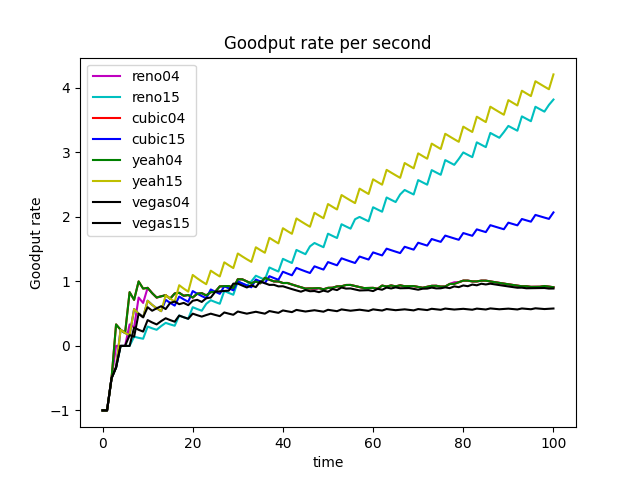
GoodPut Rate and Packet Loss Rate
Take TCP Reno Congestion Control Algorithm as an Example

TCP Reno is an extension of TCP Tahoe, and their slow start and AIMD phase are the same. In TCP Reno, the cwnd is cyclically changed in a typical situation. The cwnd continues to increase until packet loss occurs. TCP Reno has two phases in increasing its cwnd: slow start phase and congestion avoidance phase . In othrt words, TCP Reno is composed of TCP Tahoe and fast recovery (see Figure 9).
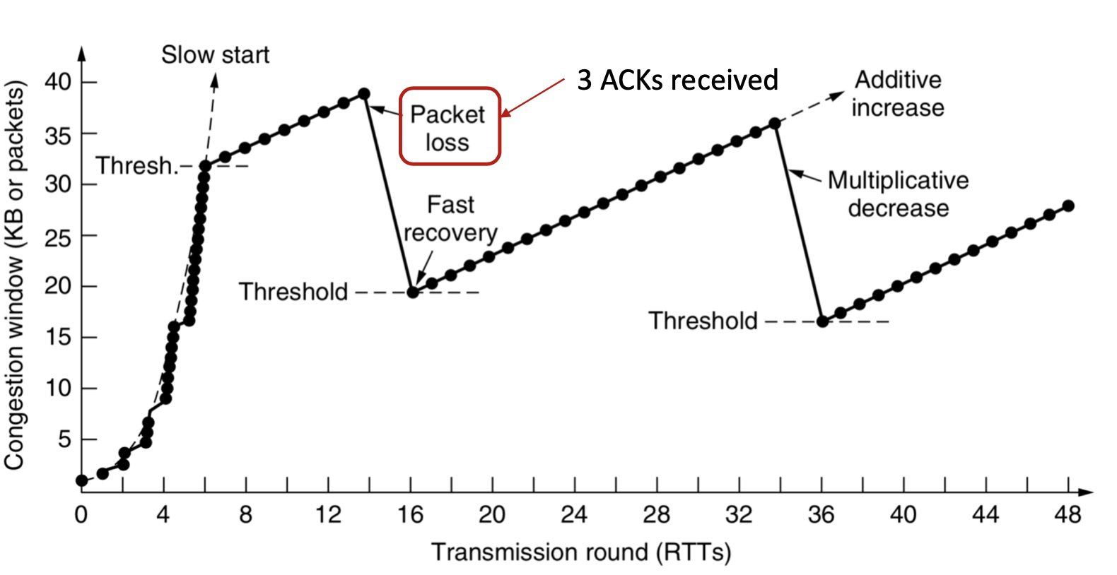

The GoodPut rate was unstable at the beginning due to the following reasons. Firstly, the beginning of the Reno algorithm is a slow start process, in which the cwnd increases exponentially, so the GoodPut rate also increases rapidly. Secondly, at around 15 seconds, the GoodPut is not stable enough because the cwnd increases too fast, and there is packet loss.
Moreover, the loss is not stable enough because, initially, the Reno algorithm needs to determine the value of cwnd based on the network conditions. Therefore, at 15 seconds, there is an excessive cwnd, which leads to packet loss.
The explanation also applies to other congestion control algorithms (Vegas, Cubic, Yeah).
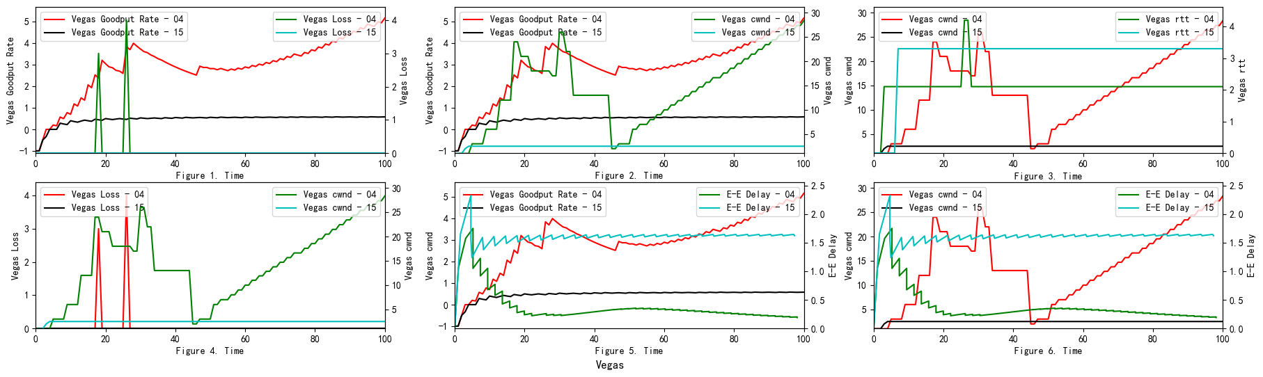
TCP Vegas
TCP Reno models can determine the network’s congestion only when packet
loss occurs in the system. In TCP Reno model, when packet loss occurs,
the window size is decreased, and the system enters the congestion
avoidance phase. While TCP Vegas senses the congestion in the network
before any packet loss occurs, it instantly decreases the cwnd.
Therefore, TCP Vegas handles the congestion without any packet loss
occurring. $Extra~Data = (expectedOutput-actualOutput)*baseRTT$
\alpha \leq (expectedOutput-actualOutput)*baseRTT \leq \beta-
If
Extra~Data > \beta, Decrease Window Size,cwnd=cwnd-1 -
If
Extra~Data < \alpha, Increase Window Size,cwnd=cwnd+1 -
If
\alpha \leq Extra~Data \leq \beta, Maintaine Window Size,cwnd=cwnd
TCP Vegas attempts to utilize the network’s bandwidth without congestion
in the network. The window size of TCP Vegas converges to the point that
lies between w + \alpha and w + \beta. TCP Vegas has congestion
control ability and also gives stability to the network, but it can not
fully use the bandwidth.
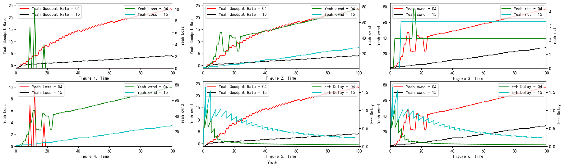
TCP YeAH
YeAH-TCP envisages two different operations: “Fast” and “Slow” modes, like Africa TCP. During the “Fast” mode, YeAH-TCP increments the cwnd according to an aggressive rule (STCP rule). In the “Slow” mode, it acts as Reno TCP.
TCP Cubic
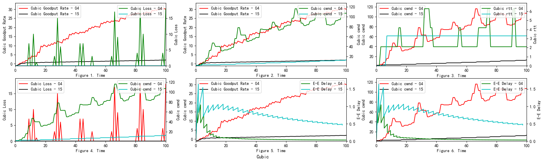
The window size in CUBIC is a cubic function of time since the most recent congestion event, with the inflection point set to the window size before the incident. The window growth function has two components because it is a cubic function. The window size quickly rises to the size prior to the most recent congestion incident in the first concave region. The convex expansion follows, where CUBIC initially searches for more bandwidth slowly and quickly. The network can stabilize because CUBIC spends a lot of time at a plateau between the concave and convex growth regions before it asks for more bandwidth.
What do you conclude after seeing these results? Which algorithm is better?
To decide which algorithm performs best, we analyze the trade-off of each algorithm at first.
Reno algorithm is a conservative algorithm, which includes slow start, congestion avoidance, fast re-transmission, and fast recovery mechanisms. The cwnd of Reno algorithm decreases quickly and grows slowly, especially in the large-window environment. It takes a long time to recover the reduced cwnd caused by the loss of a datagram. In this way, the bandwidth utilization cannot be very high, and this disadvantage will become more and more obvious with the continuous improvement of the network link bandwidth. In terms of fairness, the Reno algorithm can fairly allocate resources so that one party does not occupy a large number of resources, resulting in insufficient resources for other nodes (see Figure 8).
The Vegas algorithm takes the increase of delay RTT as the signal of network congestion. The increase of RTT leads to decreased cwnd, and the decrease of RTT leads to an increased congestion window. Specifically, Vegas adjusts the size of the congestion window by comparing the actual throughput with the expected throughput. However, Vegas algorithm is inferior to Reno in fairness. For example, it can be seen in the Figure 10 that Vegas occupies much more bandwidth on link 04 than link 15. At the same time, the overall resource utilization of the algorithm is also relatively low.
The Yeah algorithm defines two patterns. Fast mode and Slow mode, which are more aggressive in Fast mode, behave the same way as Reno in Slow mode. It solves the problem that Reno algorithm can not use all the bandwidth and ensures fair and reasonable allocation of resources. At the same time, it also has a low packet loss rate (see Figure 11).
The advantage of the Cubic algorithm is that as long as there is no packet loss, it will not actively reduce its sending speed. It can maximize the remaining bandwidth of the network, improve the throughput, and play a better performance in the network with high bandwidth and low packet loss rate. However, while the Cubic algorithm has high bandwidth utilization, it still increases the cwnd, which indirectly increases the packet loss rate (see Figure 12), resulting in the aggravation of the network jitter.
Having discussed each algorithm’s features, we now analyze which one is better.
Each algorithm has its own advantages and disadvantages and applicable scenarios. In general, the Reno algorithm and Vegas are more conservative, which is also in line with its appearance in the early days of the Internet. Yeah algorithm solves part of the problems of the Reno algorithm, but in the case of high latency and high packet loss rate for a long time into Slow mode, and Reno algorithm is consistent. The cubic algorithm is more aggressive. The Cubic algorithm is more aggressive and has a higher packet loss rate, but it can guarantee high transmission speed in a poor network environment.
How reliable are these results, and how confident are you about the conclusion you have made based on these results?
To determine to which extent these results are reliable, we need to analyze the following aspects.
-
Reliable
- The simulation is performed in a real situation setting and therefore reflects the performance of the real situation under this specific condition.
-
Unreliable
-
The given simulation only lasts 100 seconds, which means the GoodPut rate may have not converged yet. Possible convergence will occur if time extends.
-
The parameters, such as bandwidth and latency, are not random enough to demonstrate the practical situation.
-
Since the simulation adapt TCP as the only protocol, the output may have a different result when utilizing HTTP, UDP or Telnet. Therefore, further experiments are required to verify the correctness.
-
The conditions for practical situations are more complex to set than in the simulation, so the results may not be reliable or indicative.
-
The setting of practical situations may change dynamically, so the results may not be reliable or indicative.
-
The parameters of current files only include Goodput rate and loss, which are insufficient.
-
How could you improve the confidence in your results?
To find an efficient way to improve the results based on the unreliable aspects written in Section 4.2, we conducted some experiments, including randomly established parameters and extending the testing duration.
-
To alleviate the random parameters or settings, we replace the Telnet protocol with the FTP protocol by changing the following code.
set mytelnet [new Application/Telnet]
$mytelnet attach-agent $source1
Then we compare the effectiveness of each algorithm (see Figure 23).
-
We avoid the problem that the experiment may not achieve the Extending the testing duration:
Goodput of Telnet 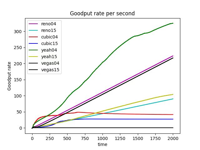
1000s - Goodput 
1000s - Loss 
Extend to 2000s Impact of the bottleneck -
We solve the disadvantage of insufficient parameters by adding more parameters (see Figure 8, 10, 11, 12)
What is the equation used in “analyser.py” to calculate the GoodPut?
We calculate the number of ACK, which can be seen as the Goodput rate
using Equation
[goo],
where N represents the Number of ACK packets, C represents Packet
size, and T represents the Measurement interval.
GoodPutRate = \frac{N \times C}{T} = \frac{d(N) \times C}{d(T)} = C \times \left(\frac{N}{T}\right)^{'}
\label{goo}$$
# Queuing Algorithms
## Impact of the bottleneck link’s queuing algorithm - DropTail and RED
<figure id="Only12">
<figure id="Only11">
<p><img src="img/WechatIMG549.jpeg" alt="image" /> <span id="Only11"
label="Only11"></span></p>
</figure>
<figure>
<img src="img/WechatIMG550.png" style="width:140.0%" />
</figure>
<figcaption>RED</figcaption>
</figure>
Random Early Detection (RED) loses packets in advance, while DropTail
only loses packets when it reaches the maximum queue limit . Here are
examples of how Cubic performs using different bottleneck link’s queuing
algorithms (see Figure
<a href="#Cubic QueueSize - DropTail" data-reference-type="ref"
data-reference="Cubic QueueSize - DropTail">21</a> and
<a href="#Cubic QueueSize - RED" data-reference-type="ref"
data-reference="Cubic QueueSize - RED">22</a>).
<figure id="Robustne1ss Analyze">
<figure id="1111">
<img src="img/WechatIMG523.png" />
<figcaption>End-to-end delay</figcaption>
</figure>
<figure id="Robustness Analyze - Telnet1">
<img src="img/WechatIMG520.jpeg" />
<figcaption>Goodput rate</figcaption>
</figure>
<figure id="222">
<img src="img/WechatIMG521.jpeg" />
<figcaption>Packet loss</figcaption>
</figure>
<figcaption>Impact of the bottleneck - RED</figcaption>
</figure>
In the given experiments setting, when we compare Figure
<a href="#1111" data-reference-type="ref" data-reference="1111">17</a>
(RED), Figure <a href="#End-to-End Delay N4" data-reference-type="ref"
data-reference="End-to-End Delay N4">1</a> (DropTail) and Figure
<a href="#End-to-End Delay N2" data-reference-type="ref"
data-reference="End-to-End Delay N2">2</a> (DropTail), we can see that
RED performs better than DropTail. This is because four different
congestion control algorithms generally have lower end-to-end delays
when using the RED bottleneck link’s queuing algorithm. Moreover, if we
compare Figure
<a href="#Cubic QueueSize - RED" data-reference-type="ref"
data-reference="Cubic QueueSize - RED">22</a> 1 (RED) and Figure
<a href="#Cubic QueueSize - DropTail" data-reference-type="ref"
data-reference="Cubic QueueSize - DropTail">21</a> 1 (DropTail), we can
see that DropTail performs better than RED in terms of Goodput rate.
<figure id="Cubic QueueSize - DropTail">
<img src="sim/QueueSize-Cubic-DropTail.png" />
<figcaption>Cubic QueueSize - DropTail</figcaption>
</figure>
<figure id="Cubic QueueSize - RED">
<img src="sim/QueueSize-Cubic-RED.png" />
<figcaption>Cubic QueueSize - RED</figcaption>
</figure>
RED adds two new mechanisms to queue management. Firstly, instead of
waiting for the queue to be full without dropping incoming packets, it
uses a probabilistic determination mechanism to drop some packets in
advance to prevent possible congestion. Secondly, it adjusts the packet
drop probability by averaging the queues instead of instant queues.
Therefore, it can absorb some transient bursts of traffic as much as
possible. Moreover, the performance of the RED algorithm is sensitive to
the design parameters and network conditions. These conditions can still
lead to multiple TCP synchronization under specific network load
conditions, resulting in throughput oscillations and increased delay
jitter.
## Repeat experiments with smaller and larger link capacity for the bottleneck link and discuss which algorithm worked better when congestion was worse
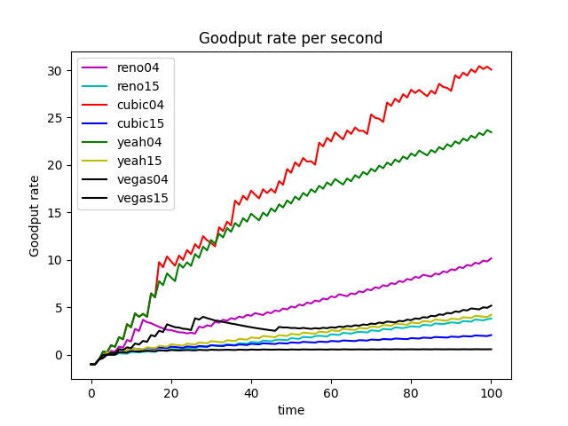
We noticed that in the given simulation scenario, the bandwidth as
1000Mb is not the bottleneck of this network (as shown in Figure
<a href="#linkspeed-test" data-reference-type="ref"
data-reference="linkspeed-test">24</a>), but the latency and queue size
significantly affect the performance of the network.
<figure id="linkspeed-test">
<figure id="Robustness Analyze - Telnet">
<img src="sim/Reno-Speed.png" />
<figcaption>Reno</figcaption>
</figure>
<figure>
<img src="sim/Cubic-speed.png" />
<figcaption>Cubic</figcaption>
</figure>
<figure>
<img src="sim/Yeah-speed.png" />
<figcaption>Yeah</figcaption>
</figure>
<figure>
<img src="sim/Cubic-speed.png" />
<figcaption>Cubic</figcaption>
</figure>
<figcaption>Throughput of 4 Algorithms</figcaption>
</figure>
In this section, we change three different simulation scenarios and show
that RED can perform much better in certain conditions.
**Setting @** is shown in the following code block. As is shown in
Figure <a href="#1mb-lower-bandwidth-RED-loss" data-reference-type="ref"
data-reference="1mb-lower-bandwidth-RED-loss">25</a> and Figure
<a href="#1mb-lower-bandwidth-DropTail-loss" data-reference-type="ref"
data-reference="1mb-lower-bandwidth-DropTail-loss">27</a>, RED performs
better than DropTail because it has a lower average loss. Moreover,
during the time interval 0-4s, all algorithms reach the highest packet
loss. Similarly, RED also performs better than DropTail because it has a
high average Goodput rate (see Figure
<a href="#1mb-lower-bandwidth-RED-goodput" data-reference-type="ref"
data-reference="1mb-lower-bandwidth-RED-goodput">26</a> and
<a href="#1mb-lower-bandwidth-DropTail-goodput"
data-reference-type="ref"
data-reference="1mb-lower-bandwidth-DropTail-goodput">28</a>).
Specifically, RED is more **stable** than DropTail, as is illustrated in
terms of both packet loss and Goodput rate (see Figure
<a href="#Simulation Scenario Setting \@slowromancap\romannumeral 1@"
data-reference-type="ref"
data-reference="Simulation Scenario Setting \@slowromancap\romannumeral 1@">29</a>).
For example, in Figure <a href="#1mb-lower-bandwidth-DropTail-goodput"
data-reference-type="ref"
data-reference="1mb-lower-bandwidth-DropTail-goodput">28</a>, Goodput
rate, when applied to the DropTail algorithm, firstly increases and
decreases when it reaches the peak at time 10s. In comparison, Goodput
rate, when applied to the RED algorithm, remains a relatively stable
high value. Therefore, in setting @, RED performs generally better than
DropTail, which can be reflected by the less packet loss and higher
Goodput rate of RED.
// It is not necessary to have a fast connection, but latency may significantly affect the network's performance.
// So we reduced the value of latency and speed; by doing this the transmission can reach the highest capacity of the bottleneck link.
$ns duplex-link $n1 $n3 4Mb 50ms DropTail
$ns duplex-link $n2 $n3 4Mb 80ms DropTail
$ns duplex-link $n3 $n4 1Mb 5ms DropTail // and RED
$ns duplex-link $n4 $n5 4Mb 50ms DropTail
$ns duplex-link $n4 $n6 4Mb 80ms DropTail
<figure id="Simulation Scenario Setting \@slowromancap\romannumeral 1@">
<figure id="1mb-lower-bandwidth-RED-loss">
<img src="img/1mb-lower-bandwidth-RED-loss.png" />
<figcaption>Loss - RED</figcaption>
</figure>
<figure id="1mb-lower-bandwidth-RED-goodput">
<img src="img/1mb-lower-bandwidth-RED-goodput.png" />
<figcaption>Goodput - RED</figcaption>
</figure>
<figure id="1mb-lower-bandwidth-DropTail-loss">
<img src="img/1mb-lower-bandwidth-DropTail-loss.png" />
<figcaption>Loss - DropTail</figcaption>
</figure>
<figure id="1mb-lower-bandwidth-DropTail-goodput">
<img src="img/1mb-lower-bandwidth-DropTail-goodput.png" />
<figcaption>Goodput - DropTail</figcaption>
</figure>
<figcaption>Simulation Scenario @</figcaption>
</figure>
**Setting @** is shown in the following code block. We also tried
another setting and saw the result. As is shown in Figure
<a href="#100queue-0.5mb-lower-bandwidth-RED-loss"
data-reference-type="ref"
data-reference="100queue-0.5mb-lower-bandwidth-RED-loss">30</a> and
<a href="#100queue-0.5mb-lower-bandwidth-DropTail-loss"
data-reference-type="ref"
data-reference="100queue-0.5mb-lower-bandwidth-DropTail-loss">32</a>,
RED performs better than DropTail since it has a relatively lower
average loss. Moreover, during the time interval 0-4s, all algorithms
reach the highest packet loss. Similarly, RED also performs better than
DropTail because it has a high average Goodput rate (see Figure
<a href="#100queue-0.5mb-lower-bandwidth-RED-goodput"
data-reference-type="ref"
data-reference="100queue-0.5mb-lower-bandwidth-RED-goodput">31</a> and
<a href="#100queue-0.5mb-lower-bandwidth-DropTail-goodput"
data-reference-type="ref"
data-reference="100queue-0.5mb-lower-bandwidth-DropTail-goodput">33</a>).
Specifically, RED is more **stable** than DropTail, as is illustrated in
terms of both packet loss and Goodput rate (see Figure
<a href="#Simulation Scenario Setting \@slowromancap\romannumeral 2@"
data-reference-type="ref"
data-reference="Simulation Scenario Setting \@slowromancap\romannumeral 2@">34</a>).
For example, in Figure
<a href="#100queue-0.5mb-lower-bandwidth-DropTail-goodput"
data-reference-type="ref"
data-reference="100queue-0.5mb-lower-bandwidth-DropTail-goodput">33</a>,
Goodput rate, when applied to the DropTail algorithm, firstly increases
and decreases when it reaches the peak at time 10s. In comparison,
Goodput rate, when applied to the RED algorithm, remains a relatively
stable high value. Therefore, in setting @, RED performs generally
better than DropTail, which can be reflected by the less packet loss and
higher Goodput rate of RED.
// RED algorithm considers the queue size. Thus, we set Queue limit to 100 and further reduced the speed of the bottleneck link.
$ns duplex-link $n1 $n3 4Mb 50ms DropTail
$ns duplex-link $n2 $n3 4Mb 80ms DropTail
$ns duplex-link $n3 $n4 0.5Mb 5ms DropTail // and RED
$ns duplex-link $n4 $n5 4Mb 50ms DropTail
$ns duplex-link $n4 $n6 4Mb 80ms DropTail
// Increase Queue Limit to 100
$ns queue-limit $n3 $n4 100
$ns queue-limit $n4 $n3 100
<figure id="Simulation Scenario Setting \@slowromancap\romannumeral 2@">
<figure id="100queue-0.5mb-lower-bandwidth-RED-loss">
<img src="question5/100queue-0.5mb-lower-bandwidth-RED-loss.png" />
<figcaption>Loss - RED</figcaption>
</figure>
<figure id="100queue-0.5mb-lower-bandwidth-RED-goodput">
<img src="question5/100queue-0.5mb-lower-bandwidth-RED-goodput.png" />
<figcaption>Goodput - RED</figcaption>
</figure>
<figure id="100queue-0.5mb-lower-bandwidth-DropTail-loss">
<img src="question5/100queue-0.5mb-lower-bandwidth-DropTail-loss.png" />
<figcaption>Loss - DropTail</figcaption>
</figure>
<figure id="100queue-0.5mb-lower-bandwidth-DropTail-goodput">
<img
src="question5/100queue-0.5mb-lower-bandwidth-DropTail-goodput.png" />
<figcaption>Goodput - DropTail</figcaption>
</figure>
<figcaption>Simulation Scenario @</figcaption>
</figure>
**Setting @** is shown in the following code block. We also try another
setting and see the result. As is shown in Figure
<a href="#largedelay500-200queue-0.5mb-lower-bandwidth-RED-loss"
data-reference-type="ref"
data-reference="largedelay500-200queue-0.5mb-lower-bandwidth-RED-loss">35</a>
and
<a href="#largedelay500-200queue-0.5mb-lower-bandwidth-DropTail-loss"
data-reference-type="ref"
data-reference="largedelay500-200queue-0.5mb-lower-bandwidth-DropTail-loss">37</a>,
RED performs better than DropTail since it has a remarkably lower loss.
Similarly, RED also performs better than DropTail because it has a high
Goodput rate (see Figure
<a href="#largedelay500-200queue-0.5mb-lower-bandwidth-RED-goodput"
data-reference-type="ref"
data-reference="largedelay500-200queue-0.5mb-lower-bandwidth-RED-goodput">36</a>
and
<a href="#largedelay500-200queue-0.5mb-lower-bandwidth-DropTail-goodput"
data-reference-type="ref"
data-reference="largedelay500-200queue-0.5mb-lower-bandwidth-DropTail-goodput">38</a>).
Specifically, RED is more **stable** than DropTail, as is illustrated in
terms of both packet loss and Goodput rate (see Figure
<a href="#Simulation Scenario Setting \@slowromancap\romannumeral 3@"
data-reference-type="ref"
data-reference="Simulation Scenario Setting \@slowromancap\romannumeral 3@">39</a>).
For example, in Figure
<a href="#largedelay500-200queue-0.5mb-lower-bandwidth-DropTail-goodput"
data-reference-type="ref"
data-reference="largedelay500-200queue-0.5mb-lower-bandwidth-DropTail-goodput">38</a>,
Goodput rate, when applied to the DropTail algorithm, firstly increases
and decreases and then shows an increasing trend again. In comparison,
Goodput rate, when applied to the RED algorithm, remains a relatively
stable ascending trend. Therefore, in setting @, RED performs generally
better than DropTail, which can be reflected by the less packet loss and
higher Goodput rate of RED.
// Here, we simulated a really poor network connection where the latency and connection speed were high.
$ns duplex-link $n1 $n3 4Mb 500ms DropTail
$ns duplex-link $n2 $n3 4Mb 800ms DropTail
$ns duplex-link $n3 $n4 0.5Mb 50ms DropTail // and RED
$ns duplex-link $n4 $n5 4Mb 500ms DropTail
$ns duplex-link $n4 $n6 4Mb 800ms DropTail
// Increase Queue Limit to 200
$ns queue-limit $n3 $n4 200
$ns queue-limit $n4 $n3 200
<figure id="Simulation Scenario Setting \@slowromancap\romannumeral 3@">
<figure id="largedelay500-200queue-0.5mb-lower-bandwidth-RED-loss">
<img
src="question5/largedelay500-200queue-0.5mb-lower-bandwidth-RED-loss.png" />
<figcaption>Loss - RED</figcaption>
</figure>
<figure id="largedelay500-200queue-0.5mb-lower-bandwidth-RED-goodput">
<img
src="question5/largedelay500-200queue-0.5mb-lower-bandwidth-RED-goodput.png" />
<figcaption>Goodput - RED</figcaption>
</figure>
<figure id="largedelay500-200queue-0.5mb-lower-bandwidth-DropTail-loss">
<img
src="question5/largedelay500-200queue-0.5mb-lower-bandwidth-DropTail-loss.png" />
<figcaption>Loss - DropTail</figcaption>
</figure>
<figure
id="largedelay500-200queue-0.5mb-lower-bandwidth-DropTail-goodput">
<img
src="question5/largedelay500-200queue-0.5mb-lower-bandwidth-DropTail-goodput.png" />
<figcaption>Goodput - DropTail</figcaption>
</figure>
<figcaption>Simulation Scenario Setting @</figcaption>
</figure>
# Conclusion
Although RED is effective in avoiding congestion, the algorithm still
suffers from the following major shortcomings. The first problem is
fairness. The RED algorithm cannot effectively handle connections that
do not respond to congestion notifications, so such connections often
crowd a large amount of network bandwidth, resulting in various
connections sharing bandwidth unfairly. Another problem is parameter
setting. The RED algorithm is sensitive to parameter settings, and small
changes in the two threshold values and the maximum packet loss
probability are often a significant impact on network performance, if
the most appropriate parameters are selected according to the specific
business environment is an important issue for RED. In addition, a set
of parameters may result in higher throughput, but may also result in
higher packet loss and longer time delays. How to configure the
parameters so that the algorithm achieves better performance in terms of
throughput, time delay, and packet loss rate also needs to be addressed.
Finally, RED also has network performance issues. The average queue
length controlled by the RED algorithm often increases as the number of
connections increases, causing transmission delay jitter and causing
unstable network performance.